YOLO

See Yolo Paper

1. Intro

Over all Sturcture/Pipeline:

1. Resize to 448 * 448
2. Conv Net
3. Threshhold the resulting detection by the model’s confidence using Non max suppression.

A single conv net simultaneously predicts multiple bounding boxes and class probabilities for those boxes. It is trained on full image and directly optimizes detection performance. Benefit over traditional method of object detection.

1. Fast. Regression problem, no need for complex pipeline. High precision
2. Reason gloabally about the image when making prediction.
3. Leans generalizable representation of objects. Less likely to break down when applied to new domain or unexpected inputs.

Drawback: Lag behind state-of-art detection system in accuracy. Struggle to precisely localize some objects. especially small ones

2. Unified Detection

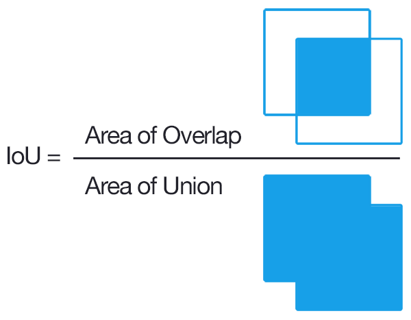
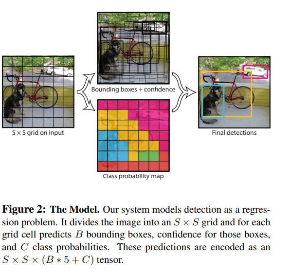
Divide the image into S * S grid. If the center of the an object falls into a grid cell, that grid cell is responsible for detecting that object. Each grid cell predicts B bounding boxes and confidence scores for those boxes. We define confidence as \(Pr(Object) * IOU_{true pred}\). IOU is between the predicted box and the groud truth.

For each bounding box (not grid cell), we have 5 prediction cell: x, y, w, h, and confidence.

• (x, y) represent the center of the box relative to the bound of the grid cell.
• (w, h) represent width and height relative to the whole image
• confidence represent IOU between the prediction box and any ground truth box.

Each grid cell (not bounding box) also predict C conditional class probabilities \(Pr(Class_i | Object)\). These probabilities are conditioned on the grid cell contraining an object. We only predict one set of class probability per grid cell, regardless of the number of the boxes.

At test time, class-specific confidence scores for each box:

\[Pr(Class_i | Object) * Pr(Object) * IOU_{true prob} = Pr(Class_i) * IOU_{true prob}\]

These score encode both

• probability of that class appearing in the bounding box
• How well the predicted box fits the object

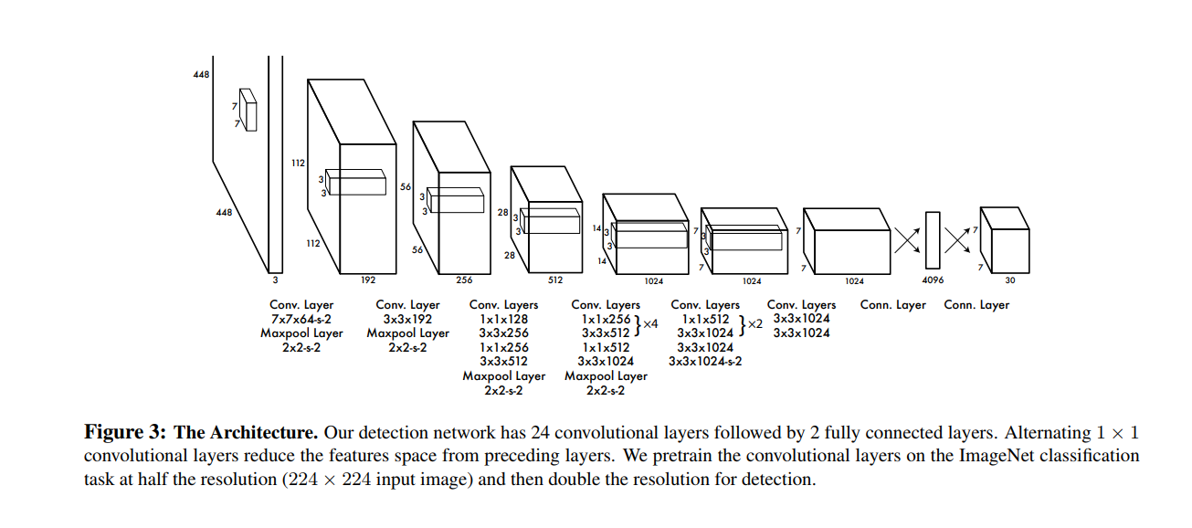
2.1 Network Desgin

2.2 Training

1. Pretrain: on ImageNet 1000-class dataset. First 20 conv layers with a fully connected layer.

2. Convert to perform detection. Add 4 Conv and 2 fully connected with randomly initiated rate. Input resolution 224 * 224 -> 448 * 448

3. Normalize witdh, height, x, y to be bounded between 0 to 1

4. Activation

   1. Final Layer: Linear Activation
   2. Other latyer: Leaky rectified linear activation function, see equation 2

5. Loss function: sum-squared error

   1. Reason: Easy to optimize
   2. Problem: (1) Does not perfectly align with our goal of maximize average precision. (2) In every image many gird cells do not contain any object. This pushes the confidence scores of those cells towards 0, often overpowering the gradient from cells that do contain object.
   3. Solution: increase loss from bounding box coordinate predictions and decrease the loss from confidence predictions from boxes that don’t contain objects. We use two parameters \(\lambda_{coord}\) = 5 and \(\lambda_{noobj}\) = 0.5
   4. Sum-squared error also equally weidgts errors in large boxes and small boxes

6. Only one bounding box should be responsible for each obejct. We assign one predictor to be responsible for predicting an object based on which prediction has the highest current IOU with the ground truth. This leads to the specialization between the bounding box prediction. Each predictor is getting better at predicting certain sizes, aspect of ratio, or class of object, improving overall recall but struglle to generalize. See the limitation of YOLO below.

1. Loss from bound box coordinate (x, y) Note that the loss comes from one bounding box from one grid cell. Even if obj not in grid cell as ground truth.

\[\begin{split}\begin{cases} \lambda_{coord} \sum^{S^2}_{i=0} [(x_i - \hat{x}_i)^2 + (y_i - \hat{y_i})^2] &\text{responsible bounding box} \\ 0 &\text{ other} \\ \end {cases}\end{split}\]

2. Loss from width w and height h. Note that the loss comes from one bounding box from one grid cell, even if the object is not in the grid cell as ground truth.

\[\begin{split}\begin {cases} \lambda_{coord} \sum^{S^2}_{i=0} [(\sqrt{w_i} - \sqrt{\hat{w}_i})^2 + (\sqrt{h_i} - \sqrt{\hat{h}_i})^2] &\text{responsible bounding box} \\ 0 &\text{ other} \\ \end {cases}\end{split}\]

3. Loss from the confidence in each bound box. Not that the loss comes from one bounding box from one grid cel, even if the object is not in the grid cell as ground truth.

\[\begin{split}\begin {cases} \sum^{S^2}_{i=0}(C_i - \hat{C}_i)^2 &\text{obj in grid cell and responsible bounding box} \\ \lambda_{noobj} \sum^{S^2}_{i=0}(C_i - \hat{C}_i)^2 &\text{obj not in grid cell and responsible bounding box} \\ 0 &\text{other} \end {cases}\end{split}\]

4. Loss from the class probability of grid cell, only when object is in the grid cell as ground truth.

\[\begin{split}\begin {cases} \sum^{S^2}_{i=0} \sum_{c \in classes} (p_i(c) - \hat{p}_i(c))^2 &\text{obj in grid cell}\\ 0 &\text{other} \\ \end {cases}\end{split}\]

Loss function only penalizes classification if obj is present in the grid cell.

It also penalize bounding box coordinate if that box is responsible for the ground box (highest IOU)

For generalization.

• Use dropout with Dropout rate 0.5.
• Data augmentation:random scaling, translation of up to 20% of the original size.
• Randomly adjust the exposure and saturation of the image by up to a factor of 1.5 in the HSV color space.

2.3 Inference

YOLO is extremely fast at test time since it only requires a single network evaluation, unlike classifier-based method.

Often it is clear which grid cell an object falls in to and the network predict one box per object. However some large objects or objects near the border of the multiple cells can be well localized by multiple cells. Non-maximal suppression can be used to fix these multiple detections.

Limitation of YOLO

• Impose strong spatial contraints on bounding box predictions since each grid cell predicts B boxes can only have one class. Limit the number of nearby objects that our model can predict. Struggles with small objetc such as flocks of birds.
• Learns to predict bounding box from data -> struggles to generalize to object in new or usual aspect ratios or configurations. Uses relatively coarse features for predicting bounding boxes since our architecture has multiple downsampling layers from the input image.
• Loss function treat error the same in small bounding boxes versus large bounding boxes. A small error in large box is generally okay but a small error in small box has a much greater effect on IOU. The main source of error comes from localization.

To understand the second limitation, revisit the paragraph from Training:

YOLO predicts multiple bounding boxes per grid cell. At training time we only want one bounding box predictor to be responsible for each object. We assign one predictor to be “responsible” for predicting an object based on which prediction has the highest current IOU with the ground truth. This leads to specialization between the bounding box predictors. Each predictor gets better at predicting certain sizes, aspect ratios, or classes of object, improving overall recall.

To understand the second limitation, consider the following example:

• Prediction on large bounding box

  • Predicted bounding box size: 16 * 16
  • Ground truth boudning box size: 25 * 25

• Prediction on large bounding box

  • Predicted bounding box size: 9 * 9
  • Ground truth boudning box size: 16 * 16

See the picture below

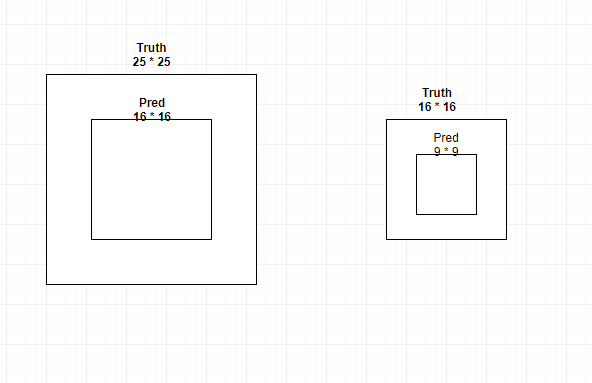
Here is the result

• Large bounding box:

  • cost on width and height: 4
  • IOU: 0.4096 <- (16 * 16) / (25 * 25)

• Small bounding box

  • cost on width and height: 4
  • IOU: 0.3164 <- (9 * 9) / (16 * 16)

The cost from the width and height of the bounding box is the same for large and small bounding box. But the IOU is not the same. The cost does not penalize the smaller IOU of the small bounding box.

Comparison to other models

• Deformable Models (DFM): Sliding window approach. Disjoint pipeline to extract features, classify regions, prediction bounding box for high scoring regions.

• RCNN: region proposal about 2000 from Selective Search. CNN extract features. SVM score the boxes. A linear model adjust the bounding box.

• Fast and faster RCNN: share computation and using Neural Network to propose region instead of Selective Search. Still fall short of real time performance.

• Deep MultiBox: predict region of interest instead of Selective Search. Cannot perform genark object detection and is still just a piece in a large detection pipeline, requiring further image classification.

• OverFeat: efficiently performs sliding window detection but it is still a disjoint system. Optimize for localization not detection performance. The localizer only see local information when making a prediction

• MultiGrasp: similar design with YOLO to work on grasp detection. Much simpler task than object detection. Only needs to prediect a single graspable region for an image containing one object. Does not have to estimate the size location or boundaries of the object or predict it’s class, om;y find a region suitable for grasping

• YOLO

  • finish the following task concurently

    • Feature extraction
    • Bound box prediction
    • Non-maximal suppression

    • YOLO is a general purpose detector that learns to detect a variety of objects simultaneously.
    • YOLO reason about global context and thus requires significant post-processing to produce coherent detection.

Resource

• Yolo Paper
• Project webpage
• RCNN Paper
• Intersection over Union IOU
• Non max suppresion
• Selective Search Paper