Focal Loss for Dense Object Detection

1. Introduction

Current state of art object detector: R-CNN framewor. Process

1. Generates a sparse set of condidate object locations
2. Classifies each condidate location as one of the foreground classes or as background

This 2-stage framework consitently achieves top accuracy on the challenging COCO benchmark.

One stage detector: YOLO, SSD. Faster with accuracy within 10-40% relative to state of art two-stage methods.

This paper: one-stage object detector, matches state of art COCO AP of more complex 2-stage detector. To achive this result, we identify imbalance during training as the main obstacle impeding 1-stage detector and propose a new loss function that eliminates this barrier.

• Class imbalance is addressed in R-CNN-like detectors by 2-stage cascade and sampling heuristics.

  1. The proposal stage rapidly narrows down the number of candidate object locatios to a small number (e.e 1-2k).
  2. In the second classification stage, sampling heuristics are performed to maintain a managable balance between foreground and background.

• 1-stage detector must process a much larger set of canidate object location regularly sampled accross an image (~ 100k locations). While similar sampling heuristics may also be applied, they are inefficient as the training procedure is still dominated by easily classifid background examples. This inefficiency is typically addressed via techniques such as bootstrapping or hard example mining.

• This paper, we propose a new loss function that act as a more effective alternative to previous approaches for dealing with class imbalance. Loss function is dynamically scaled cross entropy loss, where the scaling factor decays to 0 as confidence in the correct class increases.

This scaling factor can automatically down-weight the contribution of easy examples during training and rapidly focus the model on hard exampls. Finally we note that the exact form of the focal loss is not crucial, and we show other instantials can achive similar results.

2. Related work

• Classic object detectors: sliding window paradigm, in which a classifier is applied on dense image grid.

• 2-stage detectors

  1. generates a sparse set of condidate proposals that should contain all objects while filtering out the majority of negative locations
  2. classify the proposal into forground classes/background

• 1-stage detectors

  • Tuned for speed but accuracy trails that of two-stage method
  • 2-stage detectors can be made fast simply by reducing image resolution and number of proposal

• RetinaNet

  • shares many similarities with previous dense detector, such as anchor in RPN, features pyramids in SSD and FPN
  • simple detector achieves top results not based on innovations in design but due to novel loss.

Classic 1-stage object detection methods, and more recent methods face a large class imbalance during training. These detector evaluate \(10^4 - 10^5\) candidate locations per image but only a few location contain objects. Cause 2 problems

1. Training is inefficient as most locations are easy negatives that contributes no useful learning signal.
2. The easy negatives can overwhelm training and lead to degenerate models.

Common solution: hard negative mining that samples hard examples during training or more complex sampling/reweighing schemes.

Proposal: focal loss natually handles the class imbalance faced by one stage detector and allow us to efficiently train on all examples without sampling and without easy negatives overwhelming the loss and computed gradients.

• Robust loss: down-weighting the loss of examples with large error (hard examples).
• Focal loss: down-weighting the loss of easy examples. It focus on training in a sparse set of hard examples.

3. Focal Loss

I am not using the example of binary class in the paper, instead, I found a great explanation tutorial from here

Cross Entropy:

\[CE = - \sum y_i(log P_i)\]

Where \(y_i = 1\) if the training example belongs to class i (\(\vec{y}\) is an one-hot vector), \(P_i\) is the predicted probability. Even examples that are easily classified with \(P_i >> 0.5\) incur a loss with non-trivial magnitude. Because, even though the contribution from a single example to the loss is small, the total contribution from a large amount of examples can be non-trivial. When summed over a large number of easy examples, these small loss values can be overwhelm the rare class.

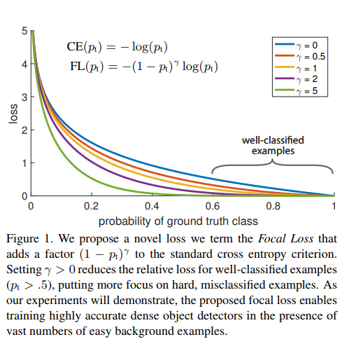
3.2 Focal Loss Definition

\[C(p, y) = - \sum y_i(1 - p_i)^\gamma \log p_i\]

\((1 - p_i)\): Modulating factor. \(\gamma\) focusing parameter.

• When the class is misclassified and \(p_i\) is small, the modulating factor is close to 1, the loss is unaffected. As \(p_i \to 1\), the factor goes to 0, the well-classified examples is down-weighted.
• The focusing paramter \(\gamma\) smoothly adjusts the rate at which easy examples are down weighted. When \(\gamma = 0\), FL is equivalent to cross entropy. As \(\gamma\) is increased the effect of the modulating fatcor is likewise increased.

In practice, we use \(\alpha-balanced\) varient of the focal loss

\[C(p, y) = - \sum y_i \alpha_i (1 - p_i)^\gamma \log p_i\]

Slightly improved accuracy over the \(non-\alpha-balanced\) form. Implementation of the loss layer combines the sigmoid operation for computing p with the loss computation, resulting in greater numerical stability.

3.3 Class Imbalance and Model Initialization

Problem: initialize equal probability to all classes, the loss due to the fequent class can domintate total loss and cause instability in the early training. Solution: introduce “prior” for the value of p etimated by the model for the rare class at the start of training. We denote the prior by \(\pi\) and set it so that the model’s estimated p for examples of the rare class is low. This improve training stability for both the cross entropy and focal loss in the case of heavy class imbalance.

3.4 Class Imbalance and 2-stage detectors

How 2-stage detector address class imbalance:

• cascase

  • reduce nearly infinite set of possible object locations down to 1000 or 2000.
  • not random, likely to correspond to true object locations, which removes vast majority of easy negatives.

• biased minibatch

  • construct mini-batch that contains, for instance, 1:3 ratio of positive and negative examples. The ratio is like an implicit \(\alpha-balance\) factor that is implemented via sampling.

4. RetinaNet Detector

• One backbone network: compute convolutional feature map over an entire image, off-the-shelf conv net.

• Two task specific subnetworks

  1. Convolutional object classification on the backbone’s output
  2. Bounding box regression

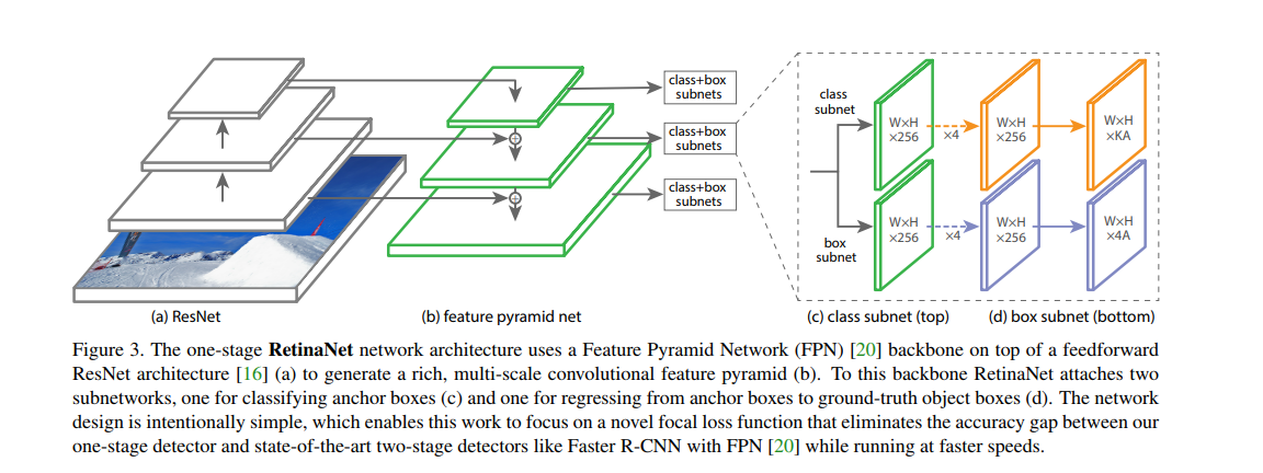
Feature Pyramid Network (FPN) Backbone: augments a std convolutional network with a top-dwon pathway and lateral connections so the network efficiently construcs a rich, multi-scale feature pyramid from a single resolution imput image. Each level of the pyramid can be used for detecting objectes at a different scale. The use of FPN backbone is preliminary; experience using features from only the final ResNet layer yield low AP.

Anchors : In total there are A = 9 anchors per level and cross levels they cover the scale range 32 - 813 pixels with respect to the network input image. Each anchor is assigned a length K one-hot vector of classification targets where K is the number of object classes, and a 4-vector of box regression targets. Anchors are assigned to ground-truth object boxes using an IoU threshold of 0.5 and to background if their IoU is in [0, 0.4). As each anchor is assigned to at most one object box, we set the corresponding entry in its length K label vector to 1 and all other entries to 0. If an anchor is unassigned, which may happen with IoY in [0.4, 0.5), it is ignored during training. Box regression targets are compued as the offset between each anchor and its assigned object box or omitted if there is no assignment.

Classification Subnets: predicts the probability of object presence at each spatial position for each of the A anchors and K object classes. This subnet is a small FCN attatched to each FPN level. parameters of this subnet are shared accross all pyramid levels. Taking an input feature map with C channels from a given pyramid level, the subnet applies 4 3 * 3 conv layers, each with C filters and each followed by RelU, followed by a 3 * 3 conv layer with KA filters. Finally sigmoid activations are attached to output the KA binary predictions per spatial location.

Box regression subnet: In parallel with the object classification subnet, we attatch another small FCN to each pyramid level for the purpose of regression the offset from each anchor box to a nearby ground-truth object. The design of the box regression subnet is identical to the classification subnet except that it ternubates in 4A linear outputs per spatial location, these 4 output predict the relatibe offset between the anchor and the ground truth box

4.1 Inference and training

Inference: Inference involves simply forwarding an image through the network. To improve speed, we only decode box predictions from at most 1k top scoring prediction per FPN level, after thresholding detector confidence at 0.05. The top predictions from all levels are merged and non-maximim suppression with a threshold of 0.5 is applied to yield the final detections.

Focal loss: it is applied to all ~100k anchors in each sampled image. The total focal loss of an image is computed as the sum of the focal loss over all ~100k anchors, normalized by the number of anchors assigned to a ground truth box. Reason: vast majority of anchors are easy negatives and receive negligible loss value value under the focal loss. In general, \(\alpha\) should be decreased slightly as \(\gamma\) is increased.

Initialization: pretrained on ImageNet 1k. All new conv layers except the final one in the RetinaNet subnets are intialized with bias b=0 and a Gaussian weight fill with \(\sigma=0.01\). For the final layer of classification subnet, we set the bias initialization to be \(b = -log((1-\pi)/\pi)\), where \(\pi\) the start of training every anchor should be labeled as foreground with confidence of \(\pi\). This init prevents the large number of background anchors from generating a large, destabilizing loss value in the first iteration of training.

<<<<<<< HEAD Optimization: trained with stochastic gradient descent (SGD). ======= ############################ 5. Experiments ############################

5.1 Training on dense detection

• Depth 50 or 101 Resnet
• Feature Pyramid Network constructed on Resnet
• 600 Pixel image

Belows are the attemps to improve the learning

1. Network Initialization

   • No modification, fail quickly
   • Simply change last layer such that the prior probability of detecting an object is 0.01 enables effective learning.

2. Use \(\alpha-balanced\) learning.

3. Use Focal Loss

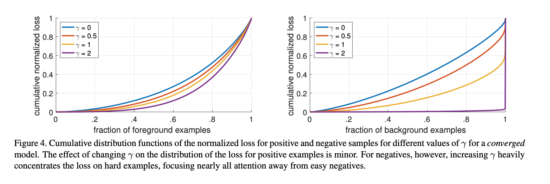
4. Analyze Focal Loss

   1. Model: Resnet-101, trained with \(\gamma = 2\)
   2. Apply this model to large number of random images
   3. Sample the predicted distribution for ~ \(10^7\) negative window and \(10^5\) postive window.
   4. Sperately for positive and negative, compute Focal Loss. Normalize the loss so that it will sum to 1.
   5. Given the normalized loss, we can sort the loss from the lowest to the highest and plot its cumulative distribution function (CDF) for both positive and negative samples and for different settings of \(\gamma\)
   6. Observed that CDF looks fairly similar for different value of \(\gamma\).
   7. Observed that CDF looks dramatically different for different value of \(\gamma\). As \(\gamma\) increases, subtantially more weights become more concentrated on the hard negative examples. With \(\gamma = 2\), vast majority of the loss comes from a small fraction of samples.

5. Online Hard Example Mining, proposed to train 2-stage detector by constructing Mini batch using high-loss examples. Result: FL is more effective than OHEM for training dense detector

   1. Each example is score by its loss
   2. Non-maximum suppression is then applied
   3. Minibatch is then constructed with highest-loss examples.
   4. Unlike FL, OHEM completely discards easy examples.

6. Hinge loss. Set loss to 0 above certain value of \(p_t\).

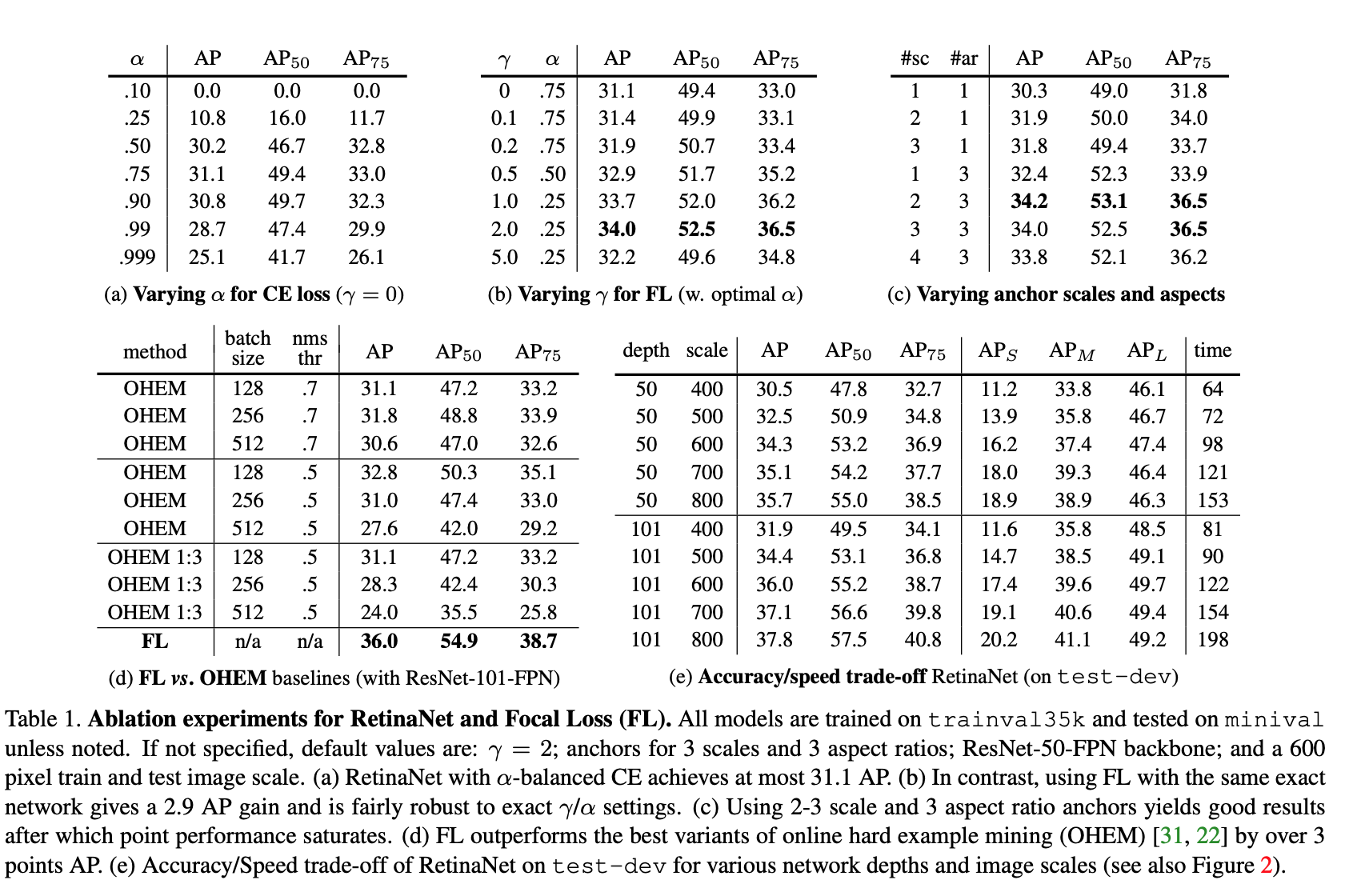
5.2 Model Architecture Design

Anchor Density: sweep over number of scales and aspect ratio anchors used at each spatial position and each pyramid level in FPN. 3 scales and 3 aspects ratio yield the best result.

Speed vs. Accuracy: larger backbone better accuracy, slower inference time.

External Resources

• RetinaNet how Focal Loss fixes Single Shot Detection
• Anchor Box
• Faster RCNN Down the rabbit hole of modern object detection
• Cumulative Distribution Function